date: 2024-09-28
title: CV-As-1
status: DONE
author:
  - AllenYGY
tags:
  - Report
  - CV
  - DFT
publish: True
Lab Report: Image Processing with 2D Discrete Fourier Transform (DFT) and Inverse DFT
Lab Overview
Resize the Image
I start by resizing the image to
   # Load the grayscale image
   img_path = "lena.jpg"  # Replace with the actual path to the image
   image = cv2.imread(img_path, cv2.IMREAD_GRAYSCALE)
   image = cv2.resize(image, (128,128))
   # Convert the image to a 2D list
   image_list = image.tolist()
Preprocess dft and idft kernel matrix
According to the formula of 2D Fourier Transform
This formula transforms the spatial domain image
- Spatial Component
- Exponential Term
This exponential term can be precomputed and stored in a 4D matrix to improve computational efficiency. By preprocessing and storing this kernel in memory, we can reuse it when calculating the DFT for each block of the image.
Take a
For an image of size
Since the similar expression between DFT and IDFT, we can also preprocess the IDFT kernel matrix in the same way.
Here is the code to preprocess the DFT and IDFT kernel matrices:
	def preprocess_dft_kernel(M, N):
	       dft_kernel = [[[[0+0j for _ in range(N)] for _ in range(M)] for _ in range(N)] for _ in range(M)]
	       for u in range(M):
	           for v in range(N):
	               for x in range(M):
	                   for y in range(N):
	                       dft_kernel[u][v][x][y] = np.exp(-2j * math.pi * ((u * x) / M + (v * y) / N))
	       return dft_kernel

	def preprocess_idft_kernel(M, N):
	       idft_kernel = [[[[0+0j for _ in range(N)] for _ in range(M)] for _ in range(N)] for _ in range(M)]
	       for u in range(M):
	           for v in range(N):
	               for x in range(M):
	                   for y in range(N):
	                       idft_kernel[u][v][x][y] = np.exp(2j * math.pi * ((u * x) / M + (v * y) / N))
	       return idft_kernel
Divide it into 256
Next, I split the resized image into
   def split_into_blocks(matrix, block_size=8):
       M = len(matrix)
       N = len(matrix[0])
       blocks = []
       for i in range(0, M, block_size):
           for j in range(0, N, block_size):
               block = [row[j:j+block_size] for row in matrix[i:i+block_size]]
               blocks.append(block)
       return blocks
   # Split image into blocks
   block_size = 8
   blocks = split_into_blocks(image_list, block_size)
Apply DFT to Each Block
By using the preprocessed DFT kernel, I apply the 2D DFT to each block to transform it into the frequency domain.
	def dft_2d(block):
	    M, N = len(block), len(block[0])
	    global dft_kernel
	    dft_result = [[0+0j for _ in range(N)] for _ in range(M)]
	    for u in range(M):
	        for v in range(N):
	            sum_val = 0
	            for x in range(M):
	                for y in range(N):
	                    sum_val += block[x][y] * dft_kernel[u][v][x][y]
	            dft_result[u][v] = sum_val
	    return dft_result

	# Preprocess DFT kernel and compute DFT for each block
	dft_kernel = preprocess_dft_kernel(block_size, block_size)
	dft_blocks = [dft_2d(block) for block in blocks]
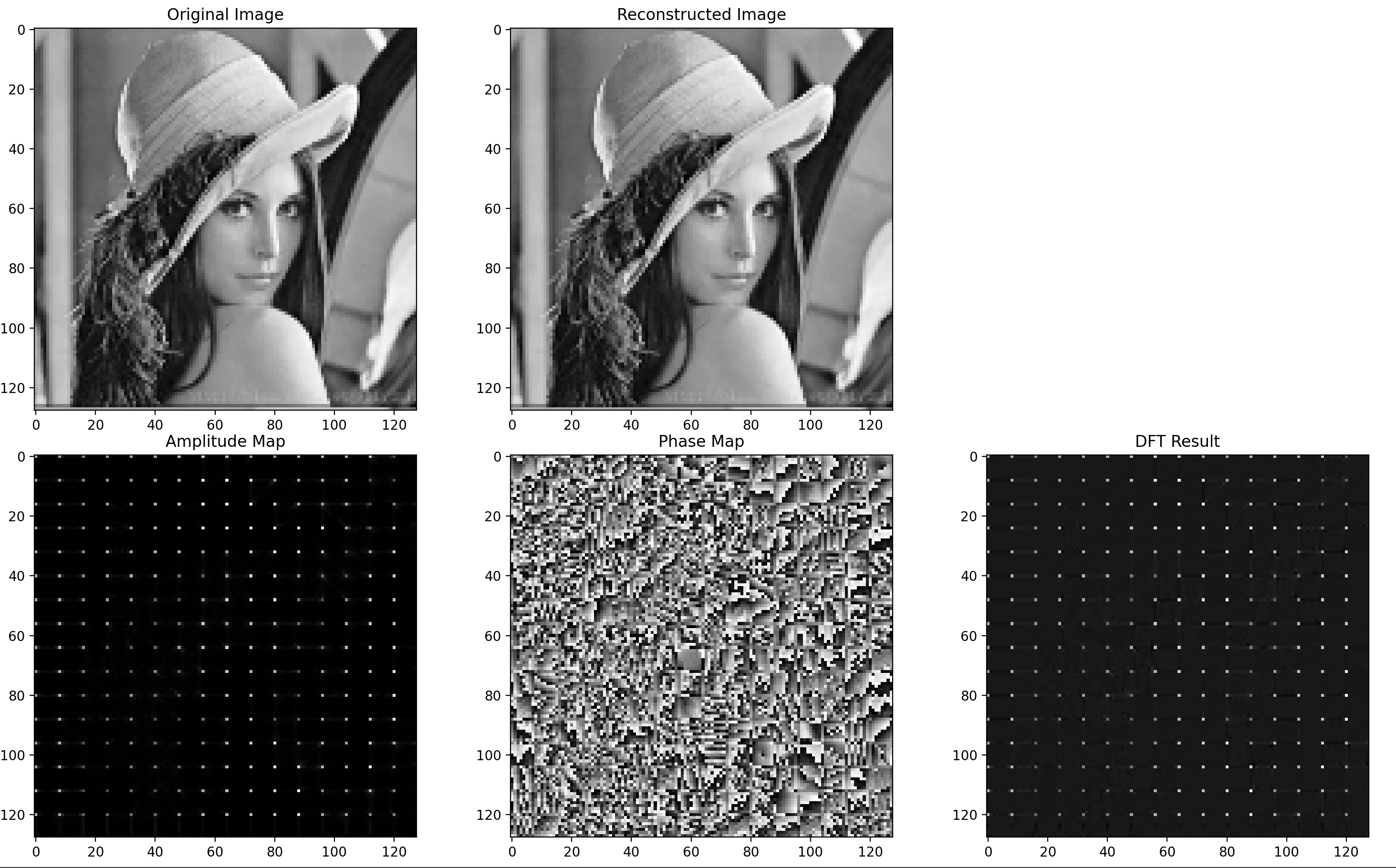
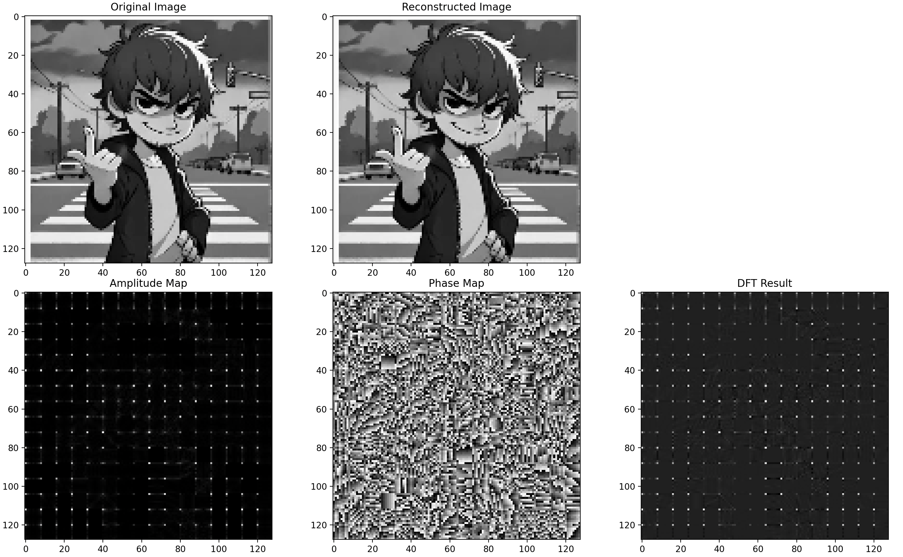
Get the Amplitude Spectrum and Phase Spectrum
The formulas in the image represent the amplitude and phase of a complex number ( F(u, v) ), typically the result of a Fourier Transform. They are given by:
Amplitude:
This is the magnitude of
Phase:
This represents the angle of ( F(u, v) ) in the complex plane, calculated as:
Here is the code to compute the amplitude and phase for each block:
	def compute_amplitude_phase(dft_block):
		M, N = len(dft_block), len(dft_block[0])
	    amplitude = [[0 for _ in range(N)] for _ in range(M)]
	    phase = [[0 for _ in range(N)] for _ in range(M)]
	    for i in range(M):
	        for j in range(N):
	            amplitude[i][j] = (dft_block[i][j].real**2 + dft_block[i][j].imag**2)**0.5
	            phase[i][j] = math.atan2(dft_block[i][j].imag, dft_block[i][j].real)
	    return amplitude, phase

	# Compute amplitude for each DFT block
	amplitude_blocks = [compute_amplitude_phase(block)[0] for block in dft_blocks]
	# Compute phase for each DFT block
	phase_blocks = [compute_amplitude_phase(block)[1] for block in dft_blocks]
Apply IDFT to Each Block
Finally, we apply the 2D IDFT to each block, transforming it back to the spatial domain.
	def idft_2d(dft_block):
	    M, N = len(dft_block), len(dft_block[0])
	    global idft_kernel
	    idft_result = [[0+0j for _ in range(N)] for _ in range(M)]
	    for x in range(M):
	        for y in range(N):
	        	sum_val = 0
	            for u in range(M):
	                for v in range(N):
	                    sum_val += dft_block[u][v] * idft_kernel[u][v][x][y]
	            idft_result[x][y] = sum_val / (M * N)
	    return idft_result

	# Preprocess IDFT kernel and compute IDFT for each DFT block
	idft_kernel = preprocess_idft_kernel(block_size, block_size)
	idft_blocks = [idft_2d(block) for block in dft_blocks]
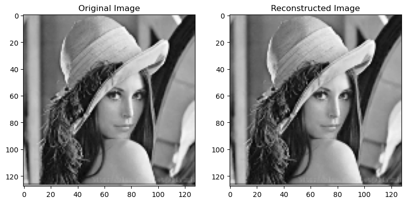
Reconstruct the Image
After applying the IDFT, I merge the blocks back by the order of division to obtain the reconstructed image and visualize the results.
   def merge_blocks(blocks, original_shape, block_size=8):
       M, N = original_shape
       merged_matrix = [[0 for _ in range(N)] for _ in range(M)]
       block_index = 0
       for i in range(0, M, block_size):
           for j in range(0, N, block_size):
               block = blocks[block_index]
               for x in range(len(block)):
                   for y in range(len(block[0])):
                       merged_matrix[i + x][j + y] = block[x][y]
               block_index += 1
       return merged_matrix

   # Merge blocks to reconstruct the image
   reconstructed_image = merge_blocks(idft_blocks, (128, 128), block_size)
   reconstructed_image_np = np.array([[z.real for z in row] for row in reconstructed_image])
Experiment Result Analysis
After dividing the (
For the reconstruction of the original image, I applied the inverse Fourier Transform to each block separately. Finally, I reassembled the blocks in their original positions, following the same layout as the initial division, to form the complete reconstructed image.
Testcase for Lena
Lena reconstructed image:
Lena DFT Phase Blocks image:
Lena DFT Amplitude Blocks image:
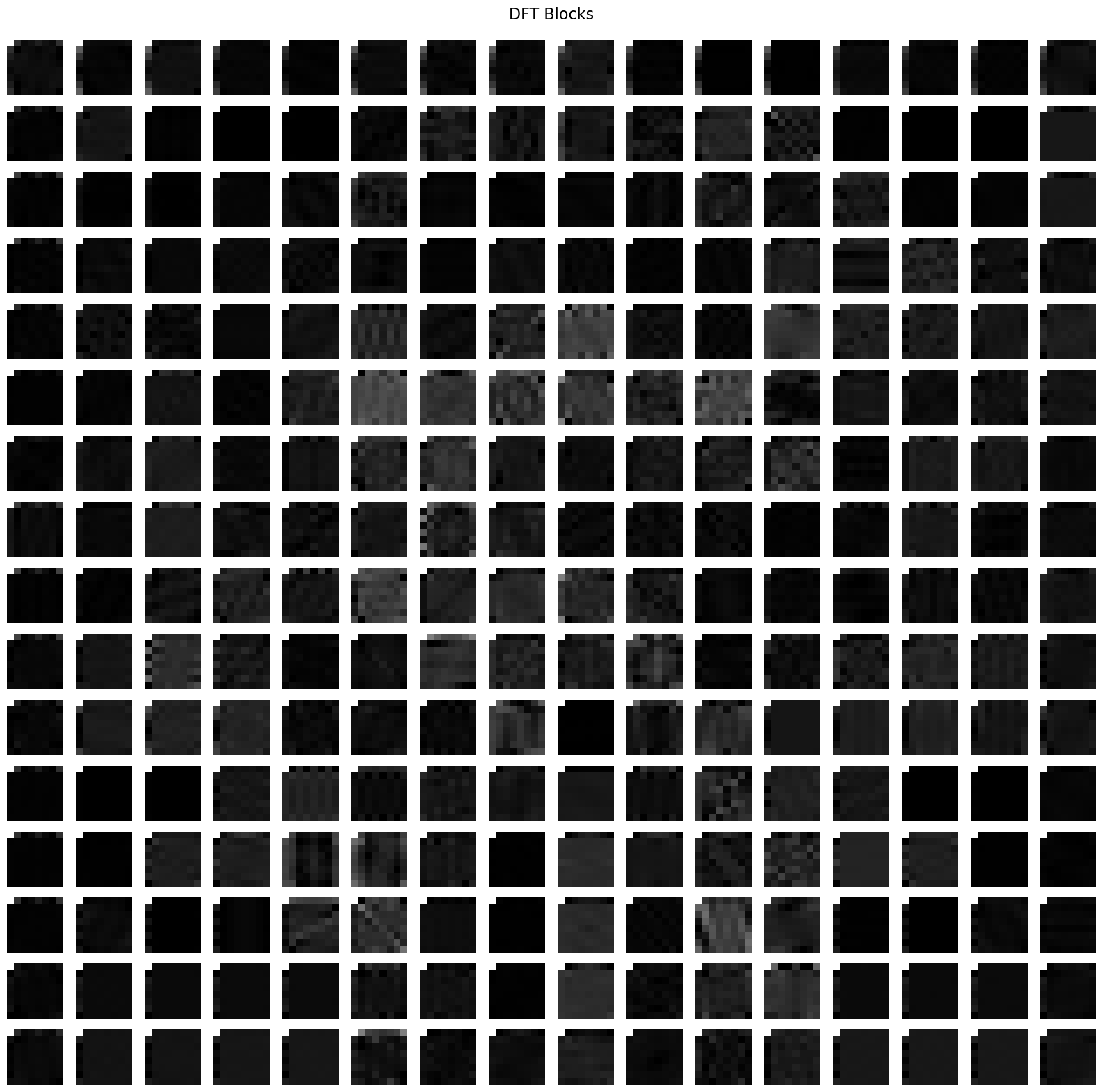
Lena DFT Blocks image:
Testcase for cartoon image
Cartoon Photo reconstructed image:
Cartoon Photo DFT Phase Blocks image:
Cartoon Photo DFT Amplitude Blocks image:
Cartoon Photo DFT Blocks image: