date: 2024-12-08
title: CV-As-3
status: DONE
author:
  - AllenYGY
tags:
  - Report
  - CV
  - ObjectDetection
publish: True
Lab Report: Object Detection Task Using LGG Dataset
Lab Overview
This lab focuses on object detection using the LGG Segmentation Dataset. The primary goal is to extract bounding boxes from segmentation masks and train an object detection model. We chose Faster R-CNN for its high accuracy and detailed feature extraction capabilities.
Data Preparation
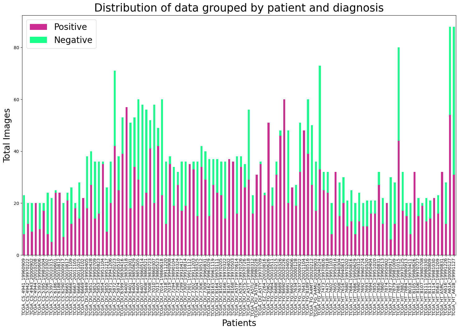
Data Distribution
Analyze the dataset to understand the proportion of slices with and without gliomas.

Generate visualizations to show class imbalance (Positive vs. Negative) and overall slice distribution.

Slice Extraction
Extract 2D slices
Process Patient Folders:
- Iterates through patient directories in the dataset.
Extract Slices:
- Loads .tif files (excluding masks) as numpy arrays using Pillow.
- Saves these arrays as PNG images to the output directory.
Output and Logging:
- Ensures output directories are created.
- Logs the file path of each saved slice.
import os
import cv2
import numpy as np
from PIL import Image

data_path = "./dataset/kaggle_3m/"
output_slices_path = "./output/slices/"
os.makedirs(output_slices_path, exist_ok=True)

for patient_folder in os.listdir(data_path):
    patient_path = os.path.join(data_path, patient_folder)
    if not os.path.isdir(patient_path):
        continue
    for file_name in os.listdir(patient_path):
        if file_name.endswith(".tif") and not file_name.endswith("_mask.tif"):
            # Load 3 chanels MRI images
            file_path = os.path.join(patient_path, file_name)
            image = np.array(Image.open(file_path))

            # save as png format
            slice_output_path = os.path.join(output_slices_path, file_name.replace(".tif", ".png"))
            cv2.imwrite(slice_output_path, image)
            print(f"Saved slice: {slice_output_path}")
Generate bounding box annotations
Process Mask Files:
- Iterates through folders, focusing on _mask.tif files.
Extract Bounding Boxes:
- Uses cv2.findContours to detect object boundaries in masks.
- Converts contours into bounding box coordinates (x_min, y_min, x_max, y_max).
Create Annotations:
- For each mask, records:
- image_id: Unique identifier.
- file_name: Corresponding PNG slice.
- bboxes: List of bounding boxes.
- category: Object class (“LGG”).
Save Annotations:
- Outputs annotations in JSON format to output_annotations_path.
import json
from PIL import Image

mask_path = "./dataset/kaggle_3m/"
output_annotations_path = "./output/annotations.json"

annotations = []
image_id = 0

for patient_folder in os.listdir(mask_path):
    patient_folder_path = os.path.join(mask_path, patient_folder)
    if not os.path.isdir(patient_folder_path):
        continue  # Skip Non-Folder

    for file_name in os.listdir(patient_folder_path):
        if file_name.endswith("_mask.tif"):  # match masked files
            # Load Mask
            mask_file_path = os.path.join(patient_folder_path, file_name)
            mask = np.array(Image.open(mask_file_path))  # Load NumPy array
        	# Find Contours
            contours, _ = cv2.findContours(mask, cv2.RETR_EXTERNAL, cv2.CHAIN_APPROX_SIMPLE)
            bboxes = []
            for contour in contours:
                x, y, w, h = cv2.boundingRect(contour)
                bboxes.append({"x_min": x, "y_min": y, "x_max": x + w, "y_max": y + h})
            if bboxes:
                # add anotation of COCO format
                annotations.append({
                    "image_id": image_id,
                    "file_name": file_name.replace("_mask.tif", ".png"),
                    "bboxes": bboxes,
                    "category": "LGG"
                })

                image_id += 1

with open(output_annotations_path, "w") as f:
    json.dump(annotations, f, indent=4)
print(f"Annotations saved to {output_annotations_path}")
Model Selection
Faster R-CNN: Known for high accuracy and detailed feature extraction.
Faster R-CNN Architecture
Faster R-CNN is a state-of-the-art object detection framework known for its high accuracy and robust feature extraction capabilities. It builds upon its predecessors (R-CNN and Fast R-CNN) by introducing a novel component called the Region Proposal Network (RPN), enabling end-to-end training and faster processing.
Architecture Overview
The Faster R-CNN architecture consists of three main components:
-
Backbone Network (Feature Extraction)
- Purpose: Extract features from the input image.
- Details:
- Typically uses a pre-trained Convolutional Neural Network (e.g., ResNet or VGG) as the backbone.
- Outputs a feature map that encodes spatial and semantic information.
- This feature map is shared across the Region Proposal Network (RPN) and Region of Interest (ROI) processing.
-
Region Proposal Network (RPN)
- Purpose: Generate region proposals (potential object locations) efficiently.
- Key Steps:
- Sliding Window: Applies a small convolutional filter (e.g., 3x3) over the feature map.
- Anchor Boxes: Predefined boxes of different sizes and aspect ratios placed at each position in the sliding window.
- Classification: Determines whether each anchor contains an object (foreground) or not (background).
- Bounding Box Regression:
- Refines anchor box coordinates to better fit the object.
- Output: A set of region proposals with scores and refined coordinates.
-
ROI Head (Region of Interest Processing)
- Purpose: Perform classification and precise bounding box regression for each region proposal.
- Key Steps:
- ROI Pooling (or ROI Align):
- Extracts fixed-size feature maps from variable-sized region proposals.
- Fully Connected Layers:
- Processes the pooled features using fully connected layers.
- Final Predictions:
- Outputs the class label and refined bounding box coordinates for each proposal.
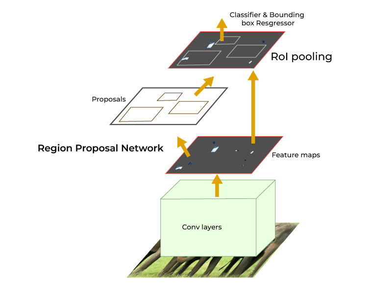
Faster R-CNN Workflow
- Input an image into the backbone network to extract feature maps.
- The RPN generates region proposals (object-like areas) from the feature maps.
- The ROI Head processes the proposals, classifying them and refining their bounding box coordinates.
- Output the final detected objects with class labels and bounding boxes.
Faster R-CNN is particularly suitable for tasks requiring high accuracy and detailed predictions, such as medical imaging, where precision is critical.
Training Process
Split the annotation dataset into training (70%), validation (20%), and testing (10%).
import json
from sklearn.model_selection import train_test_split

# Load COCO annotations
with open('./output/annotations.json', 'r') as f:
    annotations = json.load(f)

# Split dataset
train_data, temp_data = train_test_split(annotations, test_size=0.3, random_state=42)
val_data, test_data = train_test_split(temp_data, test_size=0.33, random_state=42)  # 20% val, 10% test

# Save split annotations
with open('./output/train_annotations.json', 'w') as f:
    json.dump(train_data, f)
with open('./output/val_annotations.json', 'w') as f:
    json.dump(val_data, f)
with open('./output/test_annotations.json', 'w') as f:
    json.dump(test_data, f)
Data Augmentation
Data augmentation is an essential preprocessing step to improve the robustness and generalizability of a machine learning model. By applying transformations like random horizontal flips, brightness adjustments, and other changes, the model becomes less likely to overfit and better equipped to handle variations in the input data. In this example, we define a set of augmentation transformations using PyTorch’s transforms module.
from torchvision import transforms

# Define transformations
data_transforms = transforms.Compose([
    transforms.ToTensor(),
    transforms.RandomHorizontalFlip(0.5),
    transforms.ColorJitter(brightness=0.2, contrast=0.2, saturation=0.2, hue=0.1)
])
Load Faster R-CNN Model
Faster R-CNN is a widely-used object detection model. Here, we initialize it with pre-trained weights on the COCO dataset to leverage the learned features as a starting point. The model is further customized by adjusting the box predictor to fit the specific dataset with one class of interest plus a background class. Load the Faster R-CNN model with a pre-trained backbone (e.g., ResNet50).
import torchvision
from torchvision.models.detection.faster_rcnn import FastRCNNPredictor

# Load Faster R-CNN pre-trained on COCO
model = torchvision.models.detection.fasterrcnn_resnet50_fpn(weights=True)

# Modify the box predictor to match our dataset (1 class + background)
num_classes = 2   # 1 (LGG) + 1 (background)
in_features = model.roi_heads.box_predictor.cls_score.in_features
model.roi_heads.box_predictor = FastRCNNPredictor(in_features, num_classes)
Training
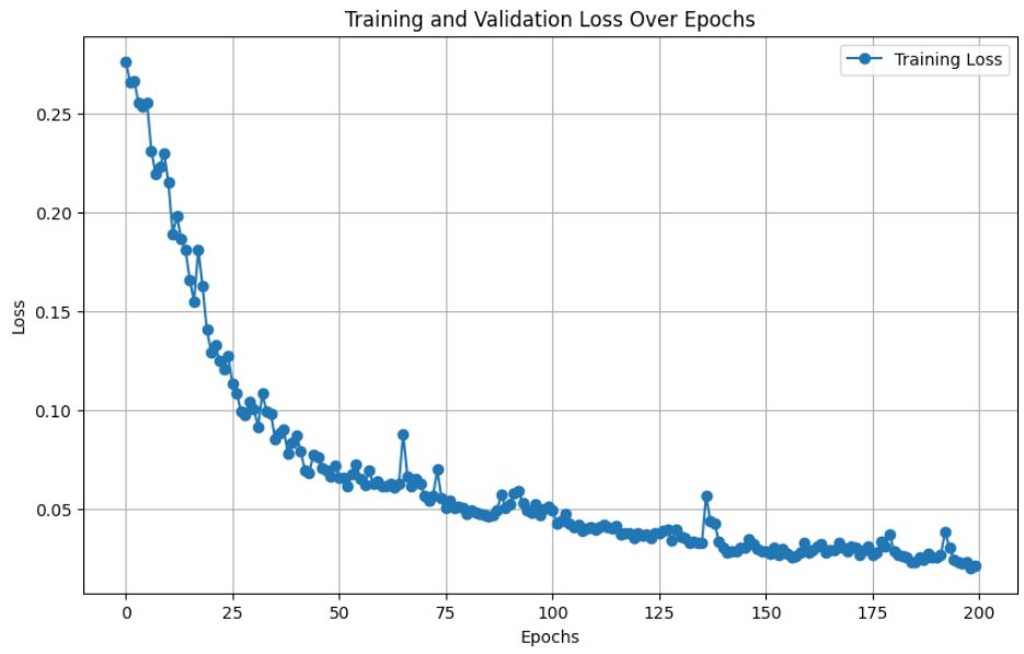
The training process involves iterating over the training dataset, feeding the data to the model, computing the loss, and updating the model parameters through backpropagation. And train for 200 epochs.
The training loop is the core process where the model learns from the data. For each batch, the model performs a forward pass to compute the loss, followed by a backward pass to update the model parameters. This implementation uses PyTorch’s gradient-based optimization process. The train_one_epoch function trains the model for one epoch, tracking the average loss for monitoring progress.
from tqdm import tqdm

def train_one_epoch(model, dataloader, optimizer, device="cpu"):
    """
    Train the Faster R-CNN model for one epoch.

    Args:
        model (torch.nn.Module): Faster R-CNN model to train.
        dataloader (torch.utils.data.DataLoader): DataLoader for training data.
        optimizer (torch.optim.Optimizer): Optimizer for training.
        device (str or torch.device): Device to run the training on (default "cpu").

    Returns:
        float: Average training loss for the epoch.
    """
    model.train()  # Set the model to training mode
    total_loss = 0  # Track total loss
    for images, targets in tqdm(dataloader, desc="Training"):
        # Move data to device
        images = [img.to(device) for img in images]
        targets = [{k: v.to(device) for k, v in t.items()} for t in targets]
        # Forward pass and compute loss
        loss_dict = model(images, targets)  # Loss dictionary
        loss = sum(loss for loss in loss_dict.values())  # Total loss
        # Backward pass and optimization
        optimizer.zero_grad()
        loss.backward()
        optimizer.step()

        total_loss += loss.item()  # Accumulate loss
    # Compute average loss
    average_loss = total_loss / len(dataloader)
    # print(f"Training Loss: {average_loss:.4f}")
    return average_loss
Validation
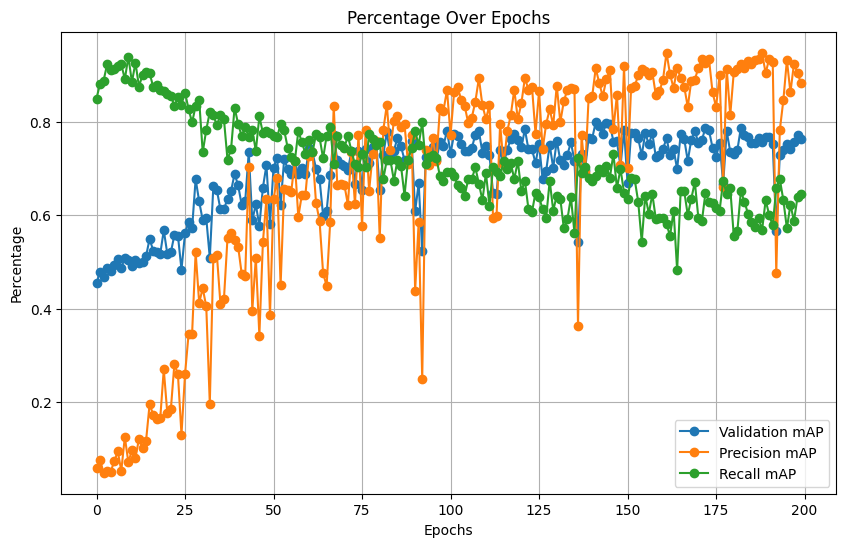
Validation assesses the performance of the model on unseen data. This function evaluates the trained model and calculates essential metrics like mean Average Precision (mAP), precision, and recall. These metrics provide insights into the model’s ability to detect objects correctly and measure its overall effectiveness. Monitor key metrics such as mean Average Precision (mAP), recall, and precision.
| mAP | Precision | Recall |
|---|---|---|
| 0.7981 | 0.8931 | 0.7031 |
def evaluate_manual_mAP(model, dataloader, device="cpu"):
    """
    Evaluate the Faster R-CNN model on the validation set and compute mAP manually.
    Args:
        model (torch.nn.Module): Faster R-CNN model to evaluate.
        dataloader (torch.utils.data.DataLoader): DataLoader for validation data.
        device (str or torch.device): Device to run the evaluation on (default "cpu").
    Returns:
        dict: Simplified metrics including mAP, precision, and recall.
    """
    model.eval()  # Set model to evaluation mode
    all_predictions = []
    all_targets = []

    with torch.no_grad():
        for images, targets in tqdm(dataloader, desc="Evaluating"):
            # Move data to device
            images = [img.to(device) for img in images]
            targets = [{k: v.to(device) for k, v in t.items()} for t in targets]
            # Forward pass to get predictions
            outputs = model(images)
            # Store predictions and targets
            all_predictions.extend(outputs)
            all_targets.extend(targets)

    # Compute mAP manually (example implementation)
    metrics = compute_metrics(all_predictions, all_targets)
    # print(f"Validation - mAP: {metrics['map']:.4f}, Precision: {metrics['precision']:.4f}, Recall: {metrics['recall']:.4f}")
    return metrics
Testing
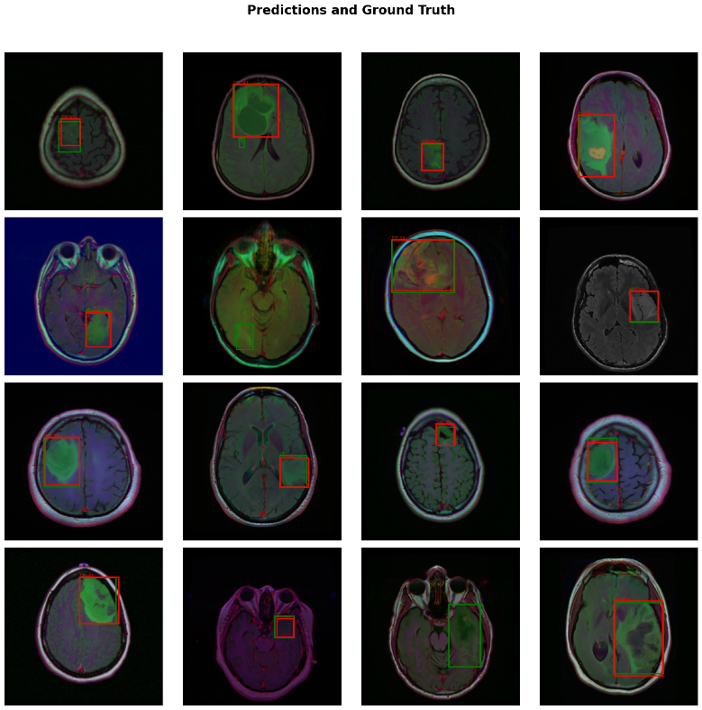
Evaluate the model on the test set and provide both quantitative metrics and qualitative outputs (detected bounding boxes overlaid on test images).
Results
import torch
from torch.optim import AdamW
from torch.utils.data import DataLoader
from torchvision.models.detection import fasterrcnn_resnet50_fpn

device = torch.device('cuda') if torch.cuda.is_available() else torch.device('cpu')
model = fasterrcnn_resnet50_fpn(weights=True).to(device)
optimizer = AdamW(model.parameters(), lr=0.0001, weight_decay=0.0001)

num_epochs = 200
train_loss_history = []
val_mAP_history=[]
val_precis_history=[]
val_recall_history=[]
best_map=-1

# Training
for epoch in range(num_epochs):
    print(f"Epoch {epoch + 1}/{num_epochs}")
    train_loss = train_one_epoch(model, train_loader, optimizer, device)
    train_loss_history.append(train_loss)
    print(f"Epoch {epoch + 1} Training Loss: {train_loss:.4f}")
    # Replace evaluate with evaluate_manual_mAP
    metrics = evaluate_manual_mAP(model, val_loader, device)
    val_mAP_history.append(metrics['map'])
    val_precis_history.append(metrics['precision'])
    val_recall_history.append(metrics['recall'])
    # Check for improvement in mAP
    if metrics['map'] > best_map:
        best_map = metrics['map']
        print(f"Validation - mAP: {metrics['map']:.4f}, Precision: {metrics['precision']:.4f}, Recall: {metrics['recall']:.4f}")
        print("New best mAP achieved! Saving model.")
        # Save the model state if mAP improves
        torch.save(model.state_dict(), 'best_model.pth')