date: 2024-11-26
title: Bioinfo-Lab-3
status: DONE
author:
  - AllenYGY
tags:
  - Lab
  - Bioinfo
publish: True
Bioinfo-Lab-3
Task 1 Filter and Normalization
import palantir
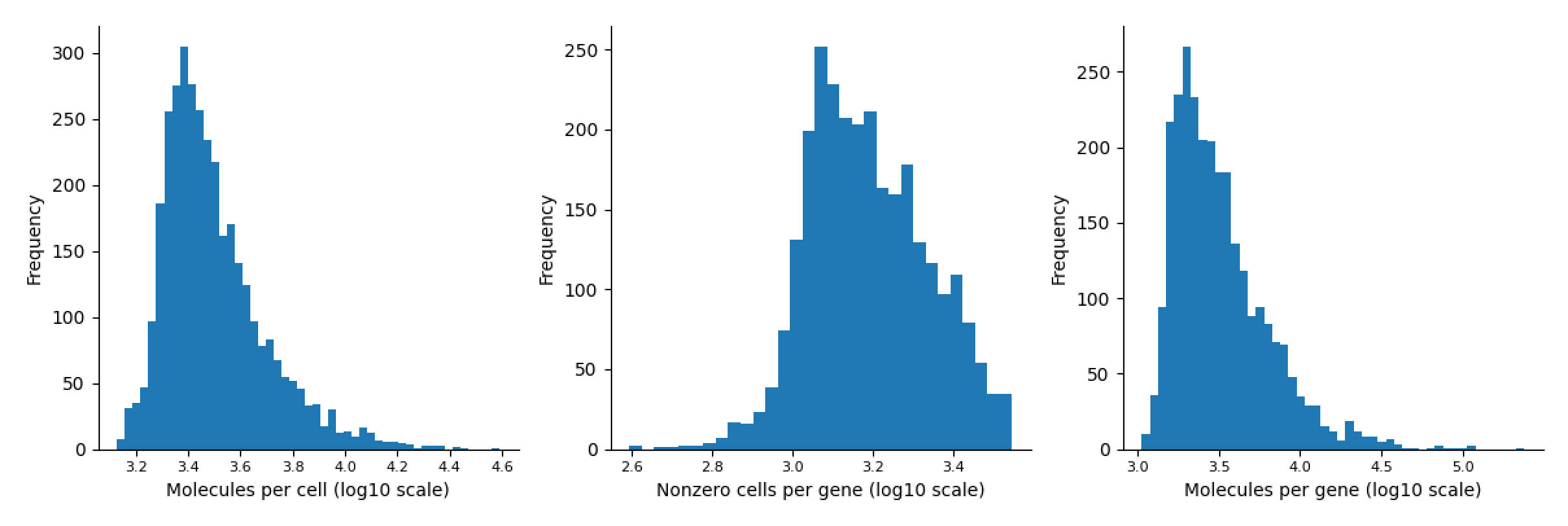
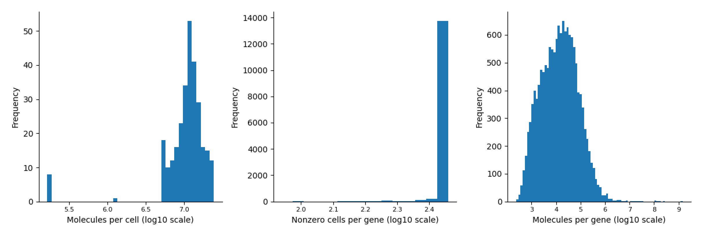
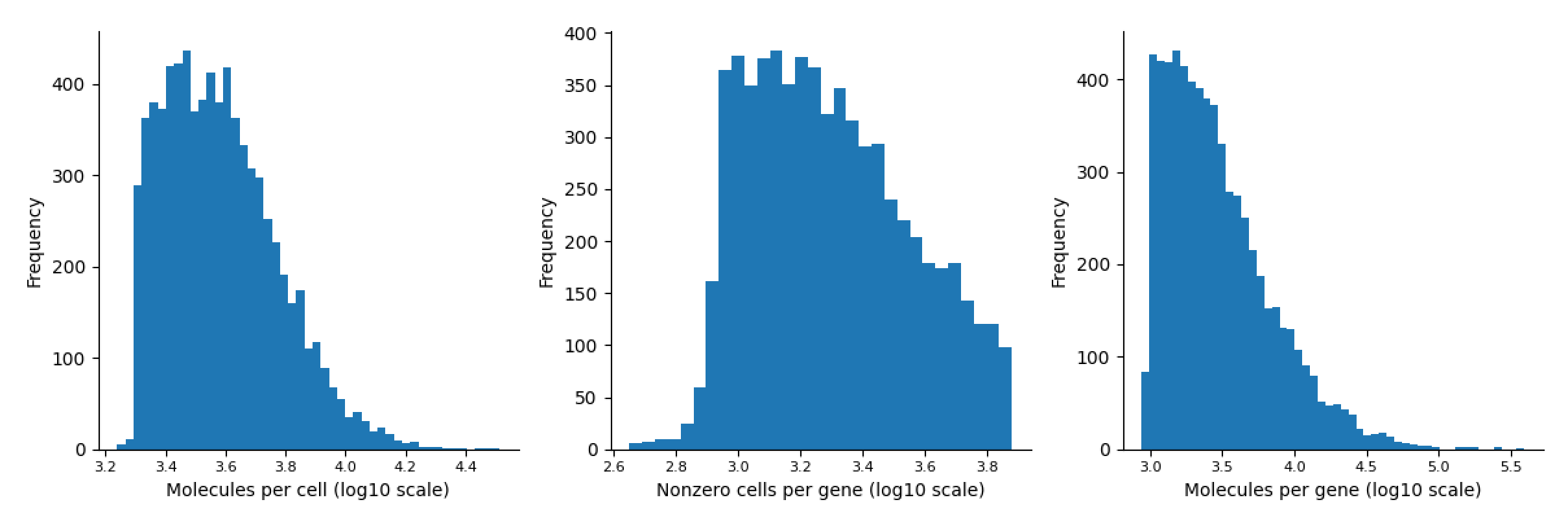
fig, ax = palantir.plot.plot_molecules_per_cell_and_gene(data.T)
filtered_data = palantir.preprocess.filter_counts_data(data.T, cell_min_molecules=1000, genes_min_cells=10)
from sklearn.preprocessing import MinMaxScaler, StandardScaler
scaler_minmax = MinMaxScaler()
data_minmax= pd.DataFrame(scaler_minmax.fit_transform(filtered_data), columns=filtered_data.columns)
print("Min-Max Scaling:")
data_minmax
scaler_zscore = StandardScaler()
data_zscore = pd.DataFrame(scaler_zscore.fit_transform(filtered_data),columns=filtered_data.columns)
print("\nZ-Score Normalization:")
data_zscore
import numpy as np
data_log = np.log(filtered_data+1)
print("Log-transformed Data:")
data_log
-
Mouse Retina Dataset
-
-
Mesc Dataset
-
-
Embryo cortex Dataset
-
Task 2 MAGIC
import magic
magic_operator=magic.MAGIC()
data_magic =magic_operator.fit_transform(data_log, genes='all_genes')
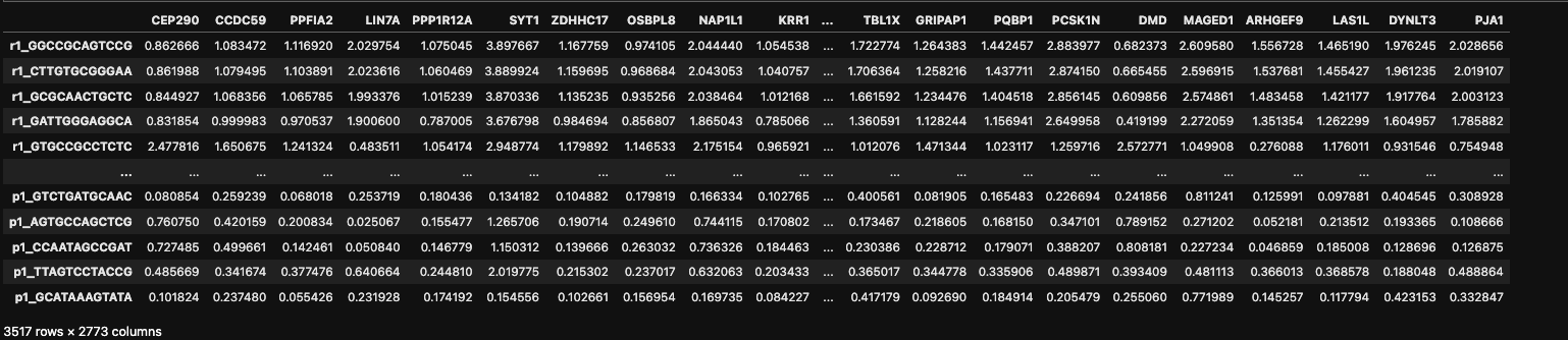
- Mouse Retina Dataset
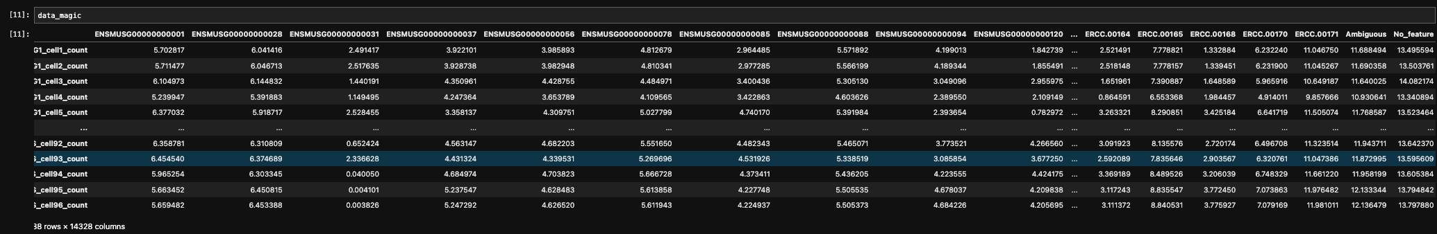
- Mesc Dataset
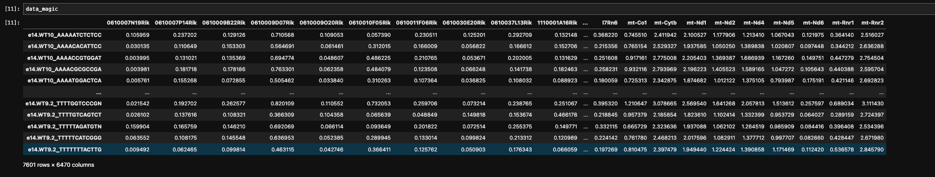
- Embryo cortex Dataset
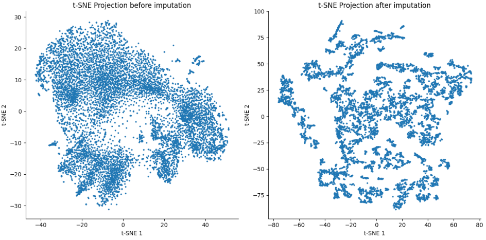
Task 3 t-SNE
from sklearn.manifold import TSNE
import matplotlib.pyplot as plt
tsne = TSNE(n_components=2)
data_tsne =tsne.fit_transform(data_log)
data_magic_tsne = tsne.fit_transform(data_magic)
import matplotlib.pyplot as plt
fig, axs = plt.subplots(1, 2, figsize=(12, 6))
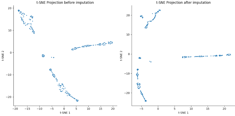
axs[0].scatter(data_tsne[:,0], data_tsne[:,1], s=3)
axs[0].set_title('t-SNE Projection before imputation')
axs[0].set_xlabel('t-SNE 1')
axs[0].set_ylabel('t-SNE 2')
axs[1].scatter(data_magic_tsne[:,0], data_magic_tsne[:,1], s=3)
axs[1].set_title('t-SNE Projection after imputation')
axs[1].set_xlabel('t-SNE 1')
axs[1].set_ylabel('t-SNE 2')
plt.tight_layout()
plt.show()
- Mouse Retina Dataset

- Mesc Dataset
- Embryo cortex Dataset
Task 4 Dimension
from sklearn.decomposition import PCA

pca = PCA(n_components=2)
data_pca =pca.fit_transform(data_log)

import umap
reducer =  umap.UMAP(n_neighbors=5)

data_umap = reducer.fit_transform(data_log)
Task 5 Clustering
from sklearn.cluster import KMeans

kmeans = KMeans(n_clusters=10)
kmeans_labels = kmeans.fit_predict(data_umap)

from sklearn.cluster import AgglomerativeClustering

model =AgglomerativeClustering(n_clusters =10, metric = 'euclidean', linkage='ward')

hierarchical_labels = model.fit_predict(data_umap)
Task 6 ARI
from sklearn.metrics import adjusted_rand_score
import pandas as pd

# ground_truth = pd.read_csv("data/data1_mouse_retina/sample_cluster_ref_filtered.txt", sep='\t', header=None, index_col=0)
# ground_truth = pd.read_csv("data/data2_mesc/sample_cluster_ref_filtered.txt", sep='\t', header=None, index_col=0)
ground_truth = pd.read_csv("data/data3_embryo_cortex/sample_cluster_ref_filtered.txt", sep=' ', header=None, index_col=0)


ground_truth.index = ground_truth.index.astype(str)
filtered_data.index = filtered_data.index.astype(str)
print(ground_truth.head())
filter_truth = ground_truth[ground_truth.index.isin(filtered_data.index)]

truth_labels = filter_truth.iloc[:, 0].values.flatten()

ari_kmeans = adjusted_rand_score(truth_labels, kmeans_labels)
ari_hierarchical = adjusted_rand_score(truth_labels, hierarchical_labels)

ari_kmeans, ari_hierarchical
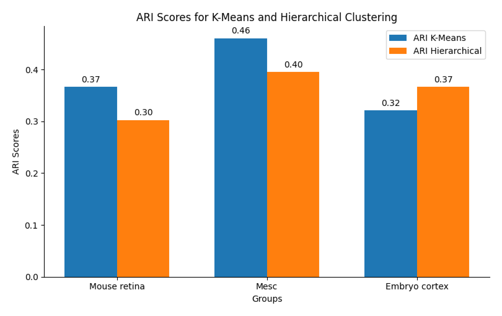
Barplot
Draw barplot to compare the ARI of different clustering method across different datasets.
import matplotlib.pyplot as plt
import numpy as np

# Data
groups = ["Mouse retina", "Mesc", "Embryo cortex"]
ari_kmeans = [ 0.3667557727356677,0.4606159477762726,0.32104987981911626]
ari_hierarchical = [0.30282121097059833,0.39561124324721736, 0.36705405669210917]

# Visualization
x = np.arange(len(groups))
width = 0.35  # Width of bars

fig, ax = plt.subplots(figsize=(8, 5))
bars1 = ax.bar(x - width/2, ari_kmeans, width, label="ARI K-Means")
bars2 = ax.bar(x + width/2, ari_hierarchical, width, label="ARI Hierarchical")

# Labels and Title
ax.set_xlabel("Groups")
ax.set_ylabel("ARI Scores")
ax.set_title("ARI Scores for K-Means and Hierarchical Clustering")
ax.set_xticks(x)
ax.set_xticklabels(groups)
ax.legend()

# Adding data labels
for bar in bars1:
    height = bar.get_height()
    ax.annotate(f'{height:.2f}', xy=(bar.get_x() + bar.get_width()/2, height),
                xytext=(0, 3), textcoords="offset points", ha='center', va='bottom')
for bar in bars2:
    height = bar.get_height()
    ax.annotate(f'{height:.2f}', xy=(bar.get_x() + bar.get_width()/2, height),
                xytext=(0, 3), textcoords="offset points", ha='center', va='bottom')

plt.tight_layout()
plt.show()