date: 2024-12-02
title: Bioinfo-Lab-4
status: DONE
author:
  - AllenYGY
tags:
  - NOTE
publish: True
Bioinfo-Lab-4
1. Reconstruct gene network adjacency matrix by Pearson correlation (see cor() in R)
data <- read.table("Gene_expression_table_filtered.txt", header=TRUE, row.names=1)
adj_matrix <- cor(data, method="pearson")
2. Draw distribution for edge weight, select edge filer cutoff.
hist(as.vector(adj_matrix), breaks=50, main="Histogram of adj", xlab="adj")
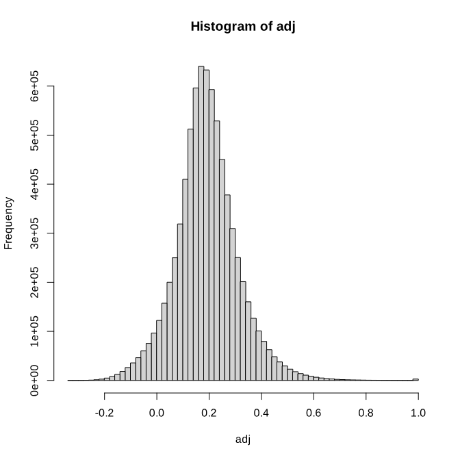
3. Keep edges whose adj(correlation)> 0.5 (see which() in R). Save adjacency edge list as a “.csv” file (see write.csv() in R, set quote=F)
A <- which(abs(adj_matrix) > 0.5, arr.ind = T)

node_list <- colnames(data)

edges <- cbind(node_list[A[, 1]], node_list[A[, 2]], adj_matrix[A])

colnames(edges) <- c("source", "target", "weight")

write.csv(edges, file = "mouse_retina_adj.csv",quote = F)
4. Convert the adjacency matrix into distance matrix by 1abs(correlation)
library(igraph)

distancematrix <- 1 - abs(adj_matrix)
5. Apply community detection (see cluster_louvain() in R package igraph).
G1 <- graph.adjacency(distancematrix, mode="undirected", weighted=TRUE, diag=TRUE)


clusterlouvain <- cluster_louvain(G1)


tmp=c()
label=c()

for (i in c(1:2)){
    tmp=c(tmp,clusterlouvain[i])
    label = c(label,rep(i,length(clusterlouvain[[i]])))
}
result=cbind(tmp,label)

write.csv(result,file="mouse_retina_node_label.csv")
6. Visualization
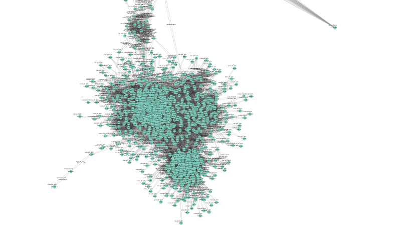
Table Of Contents